Serverless LLMs · part 6 of 7
- Anatomy of an LLM Cold Start, Part 1: Where the Time Goes
- Anatomy of an LLM Cold Start, Part 2: Make It Predictable, Then Make It Fast
- Anatomy of an LLM Cold Start, Part 3: A Checkpoint Format Written for the Reader
- ServerlessLLM Paper Breakdown, Part 1: Your GPU Server Is Also a Storage Server
- ServerlessLLM Paper Breakdown, Part 2: Migrate Tokens, Not Gigabytes
- ServerlessLLM Paper Breakdown, Part 3: Scheduling for Startup Time
- Serverless Agents: When Every Step Is a Cold Start
Two posts ago we made the storage inside GPU servers into a checkpoint cache. Last post we made it cheap to move a running inference out of the way. This post covers the scheduler, which decides for every incoming request which of those to do and where. It also covers how the whole system compares with the alternatives.
The controller
The cluster controller has two parts. The request router sends inference requests to running instances and, when none exists, hands the model loading scheduler a loading task. The scheduler owns two estimators, one for loading a model on a given server and one for migrating whatever that server is currently running. It keeps a loading task queue per server and it records every decision in a reliable key-value store such as etcd so that it can recover from its own crash.
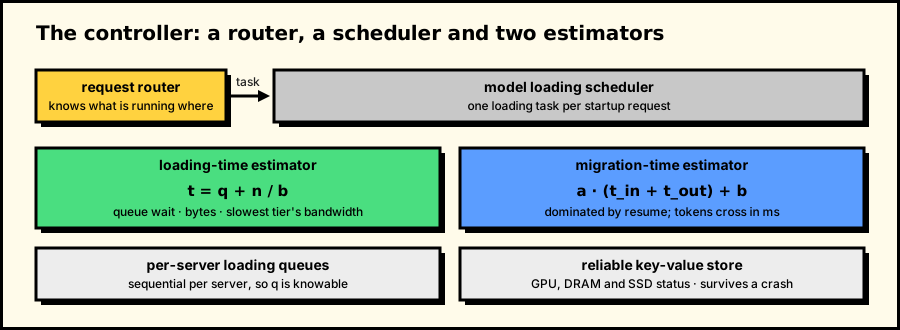
Redrawn from Figure 5 of the paper.
Estimating a load
The loading-time estimate has three inputs and one formula:
t_load = q + n / b
q is the queuing time: how long this server’s loading queue will take to drain before our task starts. n is the model size in bytes, or the partition size for a multi-GPU model. b is the bandwidth of the path the bytes will take.
Each of these involves a design decision.
q is knowable because loading is sequential per server. Both the remote-to-SSD path and the SSD-to-DRAM path are shared by every GPU on a server, so we run one loading task at a time per server and keep a single I/O queue for each path. Concurrent loads would contend for bandwidth in ways that are very hard to estimate. Sequential loads make q the sum of the estimates already in the queue. We deliberately give up some peak throughput for predictability, just as the loader does with direct I/O.
n is known before the model is opened. This is what the tiny index file from the checkpoint format is for. The scheduler reads a model’s size and partition plan from a few kilobytes of metadata, never from the weights.
b is the slowest tier involved. Because the loader pipelines across tiers, the overall time is governed by the bottleneck tier. If a model is on SSD and has to go through DRAM to the GPU, SSD bandwidth is the number, since DRAM to GPU is orders of magnitude faster. If the model is already in pinned DRAM, the PCIe link is the number. If it has to be downloaded, the network is.
The estimator does not rely on fixed bandwidth constants. Every server reports the actual latency of every load and the scheduler uses those reports to correct its per-tier bandwidth estimates over time. In the evaluation the SSD-load estimate is within about 40 ms and the GPU-side estimate within about 5 ms.
Estimating a migration
A migration’s cost is dominated by the resume step, where the destination recomputes the KV cache. Token transfer takes milliseconds, while resume takes seconds. So:
t_migrate = a * (t_in + t_out) + b
t_in is the number of prompt tokens, t_out the number of tokens generated so far and a and b are per-model constants that depend on batch size and the hardware, fitted the way LLM serving studies fit prefill cost.
Obtaining t_out raises a small systems problem. The scheduler would have to poll every server for its current output length and at thousands of scheduling decisions per second that becomes a bottleneck. Instead the scheduler asks the local request router, which already tracks the inference’s duration d and the model’s average time per token tand takes t_out = d / t. This is accurate enough and adds no traffic to the GPU servers.
When several servers could host the migrated inference, the scheduler uses a small dynamic program to pick the placement that minimises total migration time.
Choosing a server
For each server the scheduler now has the cost of loading the model from the fastest tier that holds it and the cost of migrating the current occupant and then loading from DRAM. It takes the cheaper option per server, then the cheapest server overall and returns a server id and GPU slots. If no GPU is available even after considering migration, the task is held and retried when the router reports a GPU release.
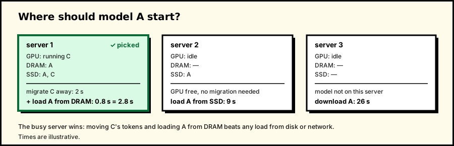
For each server, the cheaper of "load here" and "migrate what is here, then load from DRAM". Then the cheapest server. Times are illustrative.
Every step of the decision is written to the key-value store before the next step happens: GPU status on task dispatch, storage status on completion. If the scheduler dies, its replacement reads the latest server status back and resynchronises. After we made the status reads, writes and estimates asynchronous, one scheduler node handles thousands of loading tasks per second, which is plenty for the clusters we ran. Distributing the scheduler is future work.
End-to-end evaluation
The cluster evaluation ran on four servers with four A40s each, 512 GB of DRAM and one NVMe SSD per node, connected by 10 Gbps Ethernet. Since there is no public serverless LLM trace, we mapped functions from the Azure Functions trace onto models, made the arrival pattern bursty following AlpaServe and replicated OPT-6.7B, 13B and 30B into 32, 16 and 8 distinct “models” respectively. The metric is model startup latency, including any pause a migration or preemption causes.
The baselines were KServe, the standard Kubernetes serverless inference system; Ray Serve, extended to behave like a serverless platform; and Ray Serve with an LRU checkpoint cache on each server’s SSD, which is the obvious low-cost fix and gives the locality benefit without our loader or migration.
| model, dataset | ServerlessLLM | Ray Serve with cache | Ray Serve |
|---|---|---|---|
| OPT-6.7B, GSM8K | 0.8 s | 8.2 s | 12.1 s |
| OPT-30B, GSM8K | 7.5 s | 199.2 s | 213 s |
| OPT-6.7B, ShareGPT | 0.8 s | 162.4 s | 182.2 s |
| OPT-13B, ShareGPT | 1.6 s |
Average startup latency, 300-second request timeout. Even with a hypothetical 100 Gbps network, Ray Serve’s OPT-6.7B latency only drops to 3.8 s, still 4.7x ours. With OPT-30B, 89% of our requests complete inside the timeout against 26% for Ray Serve with cache. Across request rates from 0.2 to 1.1 per second on ShareGPT the improvement reaches 212x, which is where the “10 to 200x” in the abstract comes from. At 1.4 requests per second on ShareGPT with OPT-30B the GPUs are full, migration has nowhere to move inferences and our latency rises to 89.9 s. This is the limit of the approach: ServerlessLLM makes cold starts cheaper, but it cannot make up for a lack of GPUs.
KServe was slower than every Ray Serve variant, mostly because it took 114 seconds to download OPT-6.7B before it could start, for a first-token latency of 128 seconds.
Two other results convince me more than the headline number. With one GPU per server, ServerlessLLM reaches 4-second latency by migrating and swapping. Ray Serve with cache needs four GPUs per server to get down to 12 seconds. And as the number of distinct models grows with a fixed GPU count, Ray Serve with cache matches us at first and then falls behind. The system is most useful when there are many models and not enough GPUs to keep them all warm, which is the situation serverless is designed for.
Advice for practitioners
When this matters. Many models, bursty traffic and GPUs too expensive to keep every model warm. Fine-tuned variants per customer. Internal tools that are idle most of the day. Any multi-tenant platform where the model catalogue is larger than the GPU pool. In those settings a serverless design with an LLM-aware storage layer can reduce startup latency from minutes to seconds.
When it does not. One popular model under constant load. In that case it is better to keep the model resident. Cold starts are not the problem there; throughput is and that is a different research area.
Try it. The system is open source and the store can be used on its own as a fast loader. The full cluster can be started with docker compose:
curl -O https://raw.githubusercontent.com/ServerlessLLM/ServerlessLLM/main/examples/docker/docker-compose.yml
export MODEL_FOLDER=/path/to/models
docker compose up -d
docker exec sllm_head /opt/conda/envs/head/bin/sllm deploy --model Qwen/Qwen3-0.6B --backend transformers
curl http://127.0.0.1:8343/v1/chat/completions \
  -H "Content-Type: application/json" \
  -d '{"model": "Qwen/Qwen3-0.6B", "messages": [{"role": "user", "content": "What is ServerlessLLM?"}]}'
The project’s own H100 numbers today put the loader at 6 to 10x over safetensors on 32B models. It has grown past the paper: it multiplexes models on shared GPUs and serves a base model plus hundreds of LoRA adapters.
What we left open
The paper is explicit about its limitations and this post should be too. Loading is sequential per server; concurrent loading with a fairness guarantee is future work. Checkpoint placement, which server should hold which model in the first place, is treated as a separate problem and the evaluation uses round-robin. The scheduler is a single node. And the whole design assumes that a model is one thing that starts once per request.
I think the last assumption is the first to break, because many workloads today are not one model per request but pipelines of models. The final post is about this.