Serverless LLMs · part 3 of 7
- Anatomy of an LLM Cold Start, Part 1: Where the Time Goes
- Anatomy of an LLM Cold Start, Part 2: Make It Predictable, Then Make It Fast
- Anatomy of an LLM Cold Start, Part 3: A Checkpoint Format Written for the Reader
- ServerlessLLM Paper Breakdown, Part 1: Your GPU Server Is Also a Storage Server
- ServerlessLLM Paper Breakdown, Part 2: Migrate Tokens, Not Gigabytes
- ServerlessLLM Paper Breakdown, Part 3: Scheduling for Startup Time
- Serverless Agents: When Every Step Is a Cold Start
Part 2 ended with a pipelined, cache-bypassing reader that moves bytes about as fast as one Python process can. It also ended with a question: why stream 2 GiB through a ring buffer and then rebuild 201 tensors on top, when the layout we want is fixed and known before the process starts?
Changing the file format
Every optimisation so far made the reader work around a layout it did not choose: alphabetical order, unaligned tensors, a pickle to walk. Checkpoints are written once and loaded thousands of times, so the right place to spend effort is the write side. This is the ServerlessLLM checkpoint design and here it logically follows from measurements in a bottom-up approach.
The format is two files. A flat blob with tensors in forward-pass order, each starting on a 4 KiB boundary. And a tiny JSON index mapping each name to dtype, shape, offset and size.

Forward-pass order, aligned by the writer. Compare the safetensors layout in part 1.
The write side, which runs once:
ALIGN = 4096
for name in sorted(sd, key=model_order_key):   # forward-pass order, not dict order
    t = sd[name]
    nbytes = t.numel() * t.element_size()
    entries[name] = {"dtype": str(t.dtype), "shape": list(t.shape),
                     "offset": offset, "nbytes": nbytes}
    offset += (nbytes + ALIGN - 1) // ALIGN * ALIGN
The read side, which runs thousands of times, becomes four steps:
with st("read index"):
    meta = json.load(open(index))
with st("allocate 1 device buffer", sync=True):
    dev = torch.empty(meta["total_size"], dtype=torch.uint8, device=DEVICE)
with st("stream blob -> device", sync=True):
    _stream(blob, dev, total, nthreads, slab, chunk)   # part 2's pipeline
with st("build tensors (views)"):
    for name, e in meta["tensors"].items():
        sd[name] = (dev[e["offset"]:e["offset"] + e["nbytes"]]
                    .view(DTYPE[e["dtype"]])
                    .view(*e["shape"]))
Only one of these steps takes measurable time:
Loading the optimised blob
  run 1:   377.1 ms
  run 2:   331.5 ms
  run 3:   332.5 ms

  stage                                time    share
  --------------------------------------------------
  read index                         0.3 ms     0.1%
  allocate 1 device buffer           0.0 ms     0.0%
  stream blob -> device            330.7 ms    99.8%
  build tensors (views)              0.5 ms     0.1%
  --------------------------------------------------
  TOTAL                            331.5 ms   100.0%

Correctness check
  all 201 tensors bit-identical to the safetensors original

Against the external baseline
  safetensors -> mps     563.3 ms  (  3.91 GB/s)
  sllm blob   -> mps     331.5 ms  (  6.64 GB/s)
  speedup                1.70x
Constructing all 201 tensors took half a millisecond, because constructing them only involves arithmetic on offsets. There is no copy, no allocation and no access to host memory. The entire load is one allocation and one sequential pass over the file.
The padding costs almost nothing in practice: bounded by 4 KiB per tensor, 804 KiB worst case here and exactly zero for TinyLlama because every tensor is already a multiple of 4 KiB.
Why this works
Three properties, in order of how much they matter:
- The file’s layout is the destination layout. Reading it from front to back is the whole load. There is no gather step and the reader can use whatever chunk size the device likes without ever splitting a tensor.
- The index is separate and tiny. 33 KB, about 1/65,000th of the blob. A scheduler can know a model’s size and shape without opening 2 GiB of weights. This seems like a minor detail, but it is what makes cluster-level startup-time estimation possible, as the paper posts explain.
- Alignment belongs to the writer. On Linux,
O_DIRECTdemands aligned buffers and offsets. If the writer guarantees them, the reader never has to special-case a tensor.
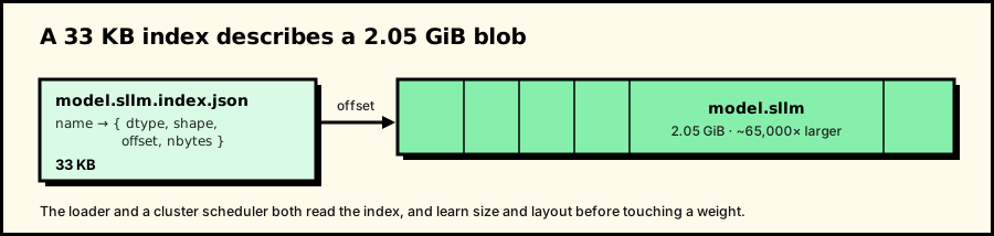
The index is the part a scheduler reads. It never has to open the weights.
The paper reports 3.6 to 8.2x over safetensors on server NVMe. I get 1.70x on a laptop whose page cache is doing half the work for safetensors. The hardware is different, but the result has the same shape and the same cause.
Results
Every loader, fresh process each, best of three, page cache warm. The first table is what a serverless worker sees. The second is steady state inside one process, for comparison with the kind of number loader benchmarks usually report.
Fresh process per load
| loader | step | time | GB/s | vs torch.load | vs safetensors |
|---|---|---|---|---|---|
| device init + allocate, no I/O | floor | 120.8 ms | 18.21 | 4.94x | 5.17x |
| torch.load(.bin) then .to(dev) | baseline | 597.0 ms | 3.69 | 1.00x | 1.05x |
| torch.load(.bin, map_location=dev) | baseline | 522.4 ms | 4.21 | 1.14x | 1.20x |
| safetensors mmap then .to(dev) | opt 1 | 925.3 ms | 2.38 | 0.65x | 0.68x |
| safetensors load_file(device=dev) | opt 1 | 625.0 ms | 3.52 | 0.96x | 1.00x |
| sllm blob, pipelined + zero-copy views | opt 4 | 390.9 ms | 5.63 | 1.53x | 1.60x |
Steady state inside one process
| loader | step | time | GB/s | vs torch.load | vs safetensors |
|---|---|---|---|---|---|
| torch.load(.bin) then .to(dev) | baseline | 437.9 ms | 5.02 | 1.00x | 1.31x |
| safetensors mmap then .to(dev) | opt 1 | 343.0 ms | 6.41 | 1.28x | 1.67x |
| safetensors load_file(device=dev) | opt 1 | 573.7 ms | 3.84 | 0.76x | 1.00x |
| sllm blob, pipelined + zero-copy views | opt 4 | 325.9 ms | 6.75 | 1.34x | 1.76x |
Why is there a gap between the tables? The “no I/O” row explains it: 121 ms of every fresh-process number is Metal building a context and handing us a 2.05 GiB buffer, before a single byte is read. Without it, the optimised loader does its actual work in about 270 ms, against a file whose physical floor on this machine is 229 ms.
This fixed cost is real, not a measurement artefact. Costs like this make serverless inference hard and they are why ServerlessLLM keeps a process warm and swaps checkpoints instead of starting a new worker per request. A constant cost cannot be optimised away, but it can be paid once instead of on every request.
A summary of the four steps:
- safetensors: mostly a safety and variance win, not a speed one.
- cache bypass: predictability and the real SSD number.
- pipelining: concurrency on the read, overlap on the copy.
- the format: removes the work the reader was doing to compensate for the layout.
Time to first token
Loader benchmarks measure the loader alone, but what matters for a user is the whole serverless worker: a process that starts, loads weights it has never touched, emits one token and exits. The last script measures exactly that, three fresh processes per loader, interleaved, prompt “The capital of France is”.
from_pretrained (safetensors)  --  best wall clock   3.471 s
  interpreter launch                 427.2 ms   12.3%
  python startup + import torch      633.5 ms   18.3%
  import transformers                1.353 s    39.0%
  tokenizer                           67.1 ms    1.9%
  from_pretrained (build + load)     799.3 ms   23.0%
  first token                        187.5 ms    5.4%    generated 'Paris'

loading-optimised blob  --  best wall clock   3.071 s
  interpreter launch                 399.7 ms   13.0%
  python startup + import torch      625.3 ms   20.4%
  import transformers                1.337 s    43.5%
  tokenizer                           61.8 ms    2.0%
  build skeleton on meta              80.7 ms    2.6%
  load weights (sllm)                406.7 ms   13.2%
  first token                        158.3 ms    5.2%    generated 'Paris'

  time to first token, from process start:
      from_pretrained           3.471 s
      loading-optimised blob    3.071 s
      saved                     399.9 ms   (1.13x end to end)
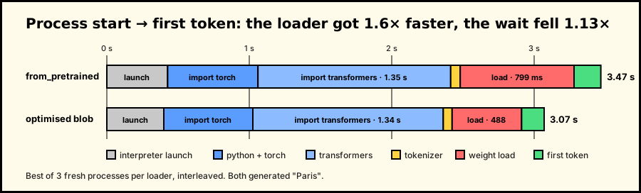
The stage we optimised got 1.64x faster. The user's wait fell 1.13x.
Loading is no longer the main cost
We made checkpoint loading 1.6x faster and the wait only fell 1.13x, because loading is no longer the biggest term:
  python + torch + transformers   1.962 s    (64% of the cold start)
  everything except loading       2.583 s    (84%)
  prefill -> first token          158.3 ms
This is Amdahl’s law and I think it is the most useful result of the three posts. Importing torch and transformers takes two seconds and no change to the checkpoint format can reduce that. What can be done is to avoid paying it on every request: keep workers warm and move the model to a warm worker instead of starting a new worker for the model.
This is a scheduling problem rather than a storage problem and it is what the paper is about. Two ideas in the paper follow directly from these numbers:
- A cluster that knows a model’s size and which storage tier holds it can predict the load time instead of discovering it. The small index file makes this possible.
- When a request would have to wait for a load, it is often cheaper to move the request’s few KB of tokens to a server that already has the weights resident and recompute the KV cache there, than to move gigabytes of weights anywhere.
Comparison with the ServerlessLLM store
Each mechanism in these three posts is a laptop-scale version of one in ServerlessLLM’s sllm_store, reached by measurement rather than taken from the paper. The numbers differ, but the reasoning is the same.
| mechanism | this series | ServerlessLLM store |
|---|---|---|
| index | model.sllm.index.json: name to dtype, shape, offset, nbytes |
tensor_index.json: name to offset, size, shape, stride, dtype |
| cache bypass | fcntl(fd, F_NOCACHE, 1) |
open(path, O_DIRECT), with a logged fallback |
| I/O concurrency | 4 Python reader threads, 64 MiB slabs | a thread pool per storage tier, configurable chunk size |
| staging | ring of 5 host buffers | pinned-memory chunk pool, DMA-capable |
| layout | one blob in model order | one sequential partition file per GPU |
| lifetime | dies with the worker | a server that outlives every worker |
The laptop cannot show the last row. Because the store outlives the worker, a second replica of a model that is already in host memory skips the disk entirely and a worker that starts on that node pays the import cost but not the load. There are also two deliberate differences: there is no pinned memory and no CUDA stream here because unified memory makes them unnecessary and the copier is one GIL-holding Python thread, which is why the pipeline turns copier-bound at eight readers where the C++ store does not.
The scope I set in part 1 still holds: single node, single model, no scheduler, no quantisation. The next posts remove the first three of these limits. Next comes the paper.